
Explore variables and build codebooks
Source:vignettes/articles/variable-exploration.Rmd
variable-exploration.RmdBefore you build frequency tables or cross-tabulations, check how your variables are named, labelled, and coded: unclear names, missing labels, unexpected codes, and variables with many missing values are easier to fix now than in a finished table. This article covers three tasks:
- recover variable labels from imported column names with
label_from_names() - inspect variables, labels, values, classes, and missing data with
varlist()andvl() - build a codebook, in the console, an Excel file, or a PDF, with
code_book()
Recover labels from imported column names
Some imported files store both a variable name and a variable label
in the column header. label_from_names() splits names of
the form name<sep>label, renames the columns, and
stores the label as a proper variable label.
df <- tibble::tibble(
  "age. Age of respondent" = c(25, 30, 41),
  "edu. Highest education level" = c("Lower", "Upper", "Tertiary"),
  "smoke. Current smoker" = c("No", "Yes", "No")
)

out <- label_from_names(df)
labelled::var_label(out)
#> $age
#> [1] "Age of respondent"
#>
#> $edu
#> [1] "Highest education level"
#>
#> $smoke
#> [1] "Current smoker"
The default separator ". " was chosen to match
LimeSurvey CSV exports taken with Export results
-> Export format: CSV -> Headings: Question code & question
text, which produce column names of the form
"code. question text". Pass sep = to use any
other literal separator.
Inspect variables with varlist()
varlist() gives a compact summary of each variable,
including its name, label, representative values, class, number of
distinct values, number of valid observations, and missing values.
In RStudio or Positron, the main way to use varlist() is
interactively. With its default behavior, it opens the overview in the
Viewer, where you can search, sort, and filter the variables.
varlist(sochealth)If you prefer a shorter call in interactive work, vl()
is a shortcut for varlist():
vl(sochealth)If you want the same summary returned as a tibble, use
tbl = TRUE:
varlist(sochealth, tbl = TRUE)
#> # A tibble: 29 × 7
#>    Variable          Label                          Values         Class N_distinct N_valid   NAs
#>    <chr>             <chr>                          <chr>          <chr>      <int>   <int> <int>
#>  1 sex               Sex                            Female, Male   fact…          2    1200     0
#>  2 age               Age (years)                    25, 26, 27, .… nume…         51    1200     0
#>  3 age_group         Age group                      25-34, 35-49,… orde…          4    1200     0
#>  4 education         Highest education level        Lower seconda… orde…          3    1200     0
#>  5 social_class      Subjective social class        Lower, Workin… orde…          5    1200     0
#>  6 region            Region of residence            Central, East… fact…          6    1200     0
#>  7 employment_status Employment status              Employed, Stu… fact…          4    1200     0
#>  8 income_group      Household income group         Low, Lower mi… orde…          4    1182    18
#>  9 income            Monthly household income (CHF) 1000, 1001, 1… nume…       1052    1200     0
#> 10 smoking           Current smoker                 No, Yes        fact…          2    1175    25
#> # ℹ 19 more rows
If you want the Values column to include explicit
missing values, use include_na = TRUE. Selecting a few
variables and keeping only the relevant columns lets the
Values strings print in full, so the added
<NA> entry is actually visible:
varlist(sochealth, smoking, income_group, self_rated_health,
  include_na = TRUE, tbl = TRUE
)[, c("Variable", "Values", "NAs")]
#> # A tibble: 3 × 3
#>   Variable          Values                                        NAs
#>   <chr>             <chr>                                       <int>
#> 1 smoking           No, Yes, <NA>                                  25
#> 2 income_group      Low, Lower middle, Upper middle, High, <NA>    18
#> 3 self_rated_health Poor, Fair, Good, Very good, <NA>              20
By default, the Values column elides longer value lists
with .... If you want to display all unique non-missing
values instead, use values = TRUE. This is especially
useful for variables with a small number of distinct values, where the
full list fits on one line. Compare the default display with the
values = TRUE display for the same two variables:
varlist(sochealth, life_sat_health, social_class,
  tbl = TRUE
)[, c("Variable", "Values", "N_distinct")]
#> # A tibble: 2 × 3
#>   Variable        Values                                          N_distinct
#>   <chr>           <chr>                                                <int>
#> 1 life_sat_health 1, 2, 3, ..., 5                                          5
#> 2 social_class    Lower, Working, Lower middle, ..., Upper middle          5

varlist(sochealth, life_sat_health, social_class,
  values = TRUE, tbl = TRUE
)[, c("Variable", "Values", "N_distinct")]
#> # A tibble: 2 × 3
#>   Variable        Values                                             N_distinct
#>   <chr>           <chr>                                                   <int>
#> 1 life_sat_health 1, 2, 3, 4, 5                                               5
#> 2 social_class    Lower, Working, Lower middle, Middle, Upper middle          5
For a focused inspection, select only the variables you want to review:
varlist(sochealth, smoking, education, income_group, tbl = TRUE)
#> # A tibble: 3 × 7
#>   Variable     Label                   Values                      Class N_distinct N_valid   NAs
#>   <chr>        <chr>                   <chr>                       <chr>      <int>   <int> <int>
#> 1 smoking      Current smoker          No, Yes                     fact…          2    1175    25
#> 2 education    Highest education level Lower secondary, Upper sec… orde…          3    1200     0
#> 3 income_group Household income group  Low, Lower middle, Upper m… orde…          4    1182    18
Declared missing values (haven’s
na_values/na_range, tagged NAs) count as
missing here too: N_valid, NAs, and
N_distinct all honor the declaration, consistently with the
tabulation functions (see the “Declared missing values” section of
?freq).
This is often enough to confirm that labels, factor levels, and missing values look correct before moving on to tabulations.
Select subsets of variables
varlist() supports tidyselect, which makes it easy to
inspect a subset of variables by name pattern or type.
varlist(sochealth, starts_with("life_sat"), tbl = TRUE)
#> # A tibble: 4 × 7
#>   Variable               Label                              Values Class N_distinct N_valid   NAs
#>   <chr>                  <chr>                              <chr>  <chr>      <int>   <int> <int>
#> 1 life_sat_health        Satisfaction with health (1-5)     1, 2,… inte…          5    1192     8
#> 2 life_sat_work          Satisfaction with work (1-5)       1, 2,… inte…          5    1192     8
#> 3 life_sat_relationships Satisfaction with relationships (… 1, 2,… inte…          5    1192     8
#> 4 life_sat_standard      Satisfaction with standard of liv… 1, 2,… inte…          5    1192     8
varlist(sochealth, where(is.numeric), tbl = TRUE)
#> # A tibble: 10 × 7
#>    Variable               Label                             Values Class N_distinct N_valid   NAs
#>    <chr>                  <chr>                             <chr>  <chr>      <int>   <int> <int>
#>  1 age                    Age (years)                       25, 2… nume…         51    1200     0
#>  2 income                 Monthly household income (CHF)    1000,… nume…       1052    1200     0
#>  3 wellbeing_score        WHO-5 wellbeing index (0-100)     18.7,… nume…        517    1200     0
#>  4 bmi                    Body mass index                   16, 1… nume…        177    1188    12
#>  5 political_position     Political position (0 = left, 10… 0, 1,… nume…         11    1185    15
#>  6 life_sat_health        Satisfaction with health (1-5)    1, 2,… inte…          5    1192     8
#>  7 life_sat_work          Satisfaction with work (1-5)      1, 2,… inte…          5    1192     8
#>  8 life_sat_relationships Satisfaction with relationships … 1, 2,… inte…          5    1192     8
#>  9 life_sat_standard      Satisfaction with standard of li… 1, 2,… inte…          5    1192     8
#> 10 weight                 Survey design weight              0.294… nume…        794    1200     0
vl() also works with tidyselect in the same way:
vl(sochealth, starts_with("bmi"), tbl = TRUE)
#> # A tibble: 2 × 7
#>   Variable     Label           Values                             Class  N_distinct N_valid   NAs
#>   <chr>        <chr>           <chr>                              <chr>       <int>   <int> <int>
#> 1 bmi          Body mass index 16, 16.6, 16.8, ..., 38.9          numer…        177    1188    12
#> 2 bmi_category BMI category    Normal weight, Overweight, Obesity order…          3    1188    12
Build a codebook
A codebook is the document that travels with a data file: what each
variable measures, how it is coded, and how many observations carry each
value. code_book() builds it from the data frame itself. It
returns an object that prints as the list of variables and that you can
keep, inspect, or write to Excel or PDF. Counts and percentages are
unweighted: they describe the data file and are not estimates for a
population.
code_book(sochealth) documents every variable. The same
tidyselect selectors as in varlist() narrow it down:
code_book(sochealth, sex, age, income_group, starts_with("bmi"))
#> Codebook
#>
#> Date: 2026-11-14
#> Observations: 1200
#> Variables: 5
#> Note: Counts and percentages are unweighted: they describe the data file and are not estimates for a population.
#>
#>    Pos. │ Variable        Label                     Type                       Valid    Missing
#> ────────┼───────────────────────────────────────────────────────────────────────────────────────
#>       1 │ sex             Sex                       categorical (nominal)       1200          0
#>       2 │ age             Age (years)               numeric                     1200          0
#>       8 │ income_group    Household income group    categorical (ordinal)       1182         18
#>      20 │ bmi             Body mass index           numeric                     1188         12
#>      21 │ bmi_category    BMI category              categorical (ordinal)       1188         12
The type is read off the R class, never guessed: a factor is
categorical (nominal), an ordered factor categorical
(ordinal), a labelled vector categorical (labelled codes),
an integer or double vector numeric, a logical, character, or
Date vector logical, text, or
date, a POSIXct or POSIXlt vector
date-time, and an hms vector time. The
level of measurement comes from the declaration alone: a factor whose
order was not declared with ordered() is nominal. A
labelled vector without value labels is numeric (or
text), like one whose labels all mark missing codes (see
below). The R class itself stays in the object.
The codebook object
Keep the result to work with its parts:
cb <- code_book(sochealth, sex, age, income_group, starts_with("bmi"))variables has one row per variable: its position in the
data frame, name, label, type, R class, valid and missing counts, the
count and codes of its declared missing values, number of distinct
values, and, for numeric variables, the minimum, maximum, mean, standard
deviation, and median (dates get their earliest and latest value
instead):
cb$variables[, c("name", "type", "n_valid", "n_missing", "n_distinct",
                 "min", "max", "mean")]
#> # A tibble: 5 × 8
#>   name         type                  n_valid n_missing n_distinct   min   max  mean
#>   <chr>        <chr>                   <int>     <int>      <int> <dbl> <dbl> <dbl>
#> 1 sex          categorical (nominal)    1200         0          2    NA  NA    NA
#> 2 age          numeric                  1200         0         51    25  75    49.3
#> 3 income_group categorical (ordinal)    1182        18          4    NA  NA    NA
#> 4 bmi          numeric                  1188        12        177    16  38.9  25.9
#> 5 bmi_category categorical (ordinal)    1188        12          3    NA  NA    NA
values has one row per category of the categorical and
logical variables, with its count and its percentages of all
observations and of the valid ones, then a row for the system missing
values (NA) of each variable that has any:
cb$values
#> # A tibble: 11 × 8
#>    position variable     code          label declared_missing     n pct_total pct_valid
#>       <int> <chr>        <chr>         <chr> <lgl>            <int>     <dbl>     <dbl>
#>  1        1 sex          Female        NA    FALSE              620      51.7      51.7
#>  2        1 sex          Male          NA    FALSE              580      48.3      48.3
#>  3        8 income_group Low           NA    FALSE              247      20.6      20.9
#>  4        8 income_group Lower middle  NA    FALSE              388      32.3      32.8
#>  5        8 income_group Upper middle  NA    FALSE              328      27.3      27.7
#>  6        8 income_group High          NA    FALSE              219      18.2      18.5
#>  7        8 income_group NA            NA    FALSE               18       1.5      NA
#>  8       21 bmi_category Normal weight NA    FALSE              465      38.8      39.1
#>  9       21 bmi_category Overweight    NA    FALSE              569      47.4      47.9
#> 10       21 bmi_category Obesity       NA    FALSE              154      12.8      13.0
#> 11       21 bmi_category NA            NA    FALSE               12       1        NA
Numeric, text, and date variables have no category rows:
variables summarizes them, and they appear in
values only through their declared missing values (see
below). An integer Likert item is numeric too: give it value labels, or
make it a factor, to list its categories. A variable with more
categories than values (100 by default), such as a list of
country or occupation codes, lists its first 100 categories in their
order, with their counts and percentages of the whole variable, then its
declared and system missing values; n_categories in
variables gives the total, and the PDF adds a row for the
categories not listed, so that its table still adds up.
values = Inf lists them all. Under the default
factor_levels = "all", unused levels count toward that
limit, and they are listed with a count of 0.
Title, subtitle, authors, and notes
The header carries what a reader needs to cite and trust the
document: a title and a subtitle, the authors with their affiliations,
the date, the numbers of observations and variables, and your notes on
the data (source, exclusions, coding rules), one note per element. In
the PDF, a note that starts with "- " is a list item,
*italics*, **bold**, and `code`
are set as such, and a web address or a doi: becomes a
link; the console and the Excel file show the words alone:
code_book(
  sochealth,
  starts_with("bmi"),
  title = "Social health survey",
  subtitle = "Body mass index",
  authors = c("Jane Doe" = "University of Somewhere"),
  notes = c(
    "Simulated data shipped with spicy (see ?sochealth).",
    "BMI in kg/m², to one decimal."
  )
)
#> Social health survey
#> Body mass index
#> Jane Doe – University of Somewhere
#>
#> Date: 2026-11-14
#> Observations: 1200
#> Variables: 2
#> Note: Counts and percentages are unweighted: they describe the data file and are not estimates for a population.
#> Note: Simulated data shipped with spicy (see ?sochealth).
#> Note: BMI in kg/m², to one decimal.
#>
#>    Pos. │ Variable        Label              Type                       Valid    Missing
#> ────────┼────────────────────────────────────────────────────────────────────────────────
#>      20 │ bmi             Body mass index    numeric                     1188         12
#>      21 │ bmi_category    BMI category       categorical (ordinal)       1188         12
authors also accepts a list of lists with
name, affiliation, and orcid.
When the variables were renamed after import, source
records the code each one had in the source file, such as a LimeSurvey
question code: with sex and age selected,
source = c(sex = "Q1", age = "Q2") fills the
source column of variables.
The words the codebook adds (column headers, types, header fields)
follow options(spicy.language): set it to "fr"
for a French codebook. The labels of the data are never translated.
Declared missing values
Data imported from SPSS often declare missing codes, such as 8 =
Don’t know and 9 = Refused.
haven::read_sav() keeps them only with
user_na = TRUE: its default turns them into
NA. Stata files carry extended missing values
(.a, .b, …) instead, which haven reads as
tagged NAs. code_book() honors both
declarations as the tabulation functions do (see the “Declared missing
values” section of ?freq): the declared codes count as
missing, are listed in values with
declared_missing = TRUE, and are summarized in the header
with the variables that carry them.
trust <- haven::labelled_spss(
  c(1, 2, 2, 3, 4, 8, 9, 1, NA, 2),
  labels = c(
    "Not at all" = 1, "A little" = 2, "Somewhat" = 3, "A lot" = 4,
    "Don't know" = 8, "Refused" = 9
  ),
  na_values = c(8, 9),
  label = "Trust in the health system"
)
income <- haven::labelled_spss(
  c(3200, 4100, 99998, 5600, 99999, 2900, NA, 7400, 3800, 4500),
  labels = c("Don't know" = 99998, "Refused" = 99999),
  na_values = c(99998, 99999),
  label = "Monthly household income (CHF)"
)

cbi <- code_book(tibble::tibble(trust, income))
cbi
#> Codebook
#>
#> Date: 2026-11-14
#> Observations: 10
#> Variables: 2
#> Declared missing value: 8 = Don't know (1 variable)
#> Declared missing value: 9 = Refused (1 variable)
#> Declared missing value: 99998 = Don't know (1 variable)
#> Declared missing value: 99999 = Refused (1 variable)
#> Note: Counts and percentages are unweighted: they describe the data file and are not estimates for a population.
#>
#>    Pos. │ Variable    Label                   Type                              Valid    Missing
#> ────────┼────────────────────────────────────────────────────────────────────────────────────────
#>       1 │ trust       Trust in the health…    categorical (labelled codes)          7          3
#>       2 │ income      Monthly household i…    numeric                               7          3
cbi$values
#> # A tibble: 10 × 8
#>    position variable code  label      declared_missing     n pct_total pct_valid
#>       <int> <chr>    <chr> <chr>      <lgl>            <int>     <dbl>     <dbl>
#>  1        1 trust    1     Not at all FALSE                2        20      28.6
#>  2        1 trust    2     A little   FALSE                3        30      42.9
#>  3        1 trust    3     Somewhat   FALSE                1        10      14.3
#>  4        1 trust    4     A lot      FALSE                1        10      14.3
#>  5        1 trust    8     Don't know TRUE                 1        10      NA
#>  6        1 trust    9     Refused    TRUE                 1        10      NA
#>  7        1 trust    NA    NA         FALSE                1        10      NA
#>  8        2 income   99998 Don't know TRUE                 1        10      NA
#>  9        2 income   99999 Refused    TRUE                 1        10      NA
#> 10        2 income   NA    NA         FALSE                1        10      NA
cbi$variables[, c("name", "type", "declared_codes", "min", "max", "mean")]
#> # A tibble: 2 × 6
#>   name   type                         declared_codes   min   max  mean
#>   <chr>  <chr>                        <chr>          <dbl> <dbl> <dbl>
#> 1 trust  categorical (labelled codes) 8, 9              NA    NA    NA
#> 2 income numeric                      99998, 99999    2900  7400  4500
trust has labels on its valid codes: it is
categorical (labelled codes), and values lists its
four answers, then its two declared missing codes and its system missing
value. Every value label of income sits on a declared
missing code and its valid values are measurements, so
code_book() reads it as numeric: its statistics
are computed on the valid values, and its only rows in
values are its missing values. With
user_na = FALSE, the declaration is ignored: the declared
codes count as valid values, and income becomes a
categorical variable whose every observed amount is a category.
Write the codebook to Excel
output = "<path>.xlsx" writes the codebook to an
Excel workbook (this needs the openxlsx2 package): a first
worksheet with the header, then the variables and
values tables. Each table starts on row 1 with a frozen
header and filters, so it sorts cleanly and reads back without skipping
rows. Numbers stay numeric cells, and dates are text.
Write the codebook to PDF
output = "<path>.pdf" writes the codebook as a
document to share: a cover (title, subtitle, authors, date), a page
about the data (numbers of observations and variables, notes, declared
missing values), the list of variables with their pages, one sheet per
variable, and an index of the variables sorted by name. It needs the
quarto package and Quarto 1.7 or later, whose bundled Typst compiles the
PDF. Without Quarto, output = "<path>.typ" writes the
Typst source, which typst compile turns into the same PDF
on any machine with Typst 0.12 or later. paper = "letter"
changes the paper size, font, font_code, and
colors the look, and index_columns the index
of variables, which takes two columns past 40 variables unless told
otherwise. spicy does not write DDI-XML: for a DDI description of the
data file, see the DDIwR package.
The call below produced the codebook of sochealth that
the package site serves: the
PDF, the
same in French (the words of the codebook, under
options(spicy.language = "fr")), and the
Excel workbook.
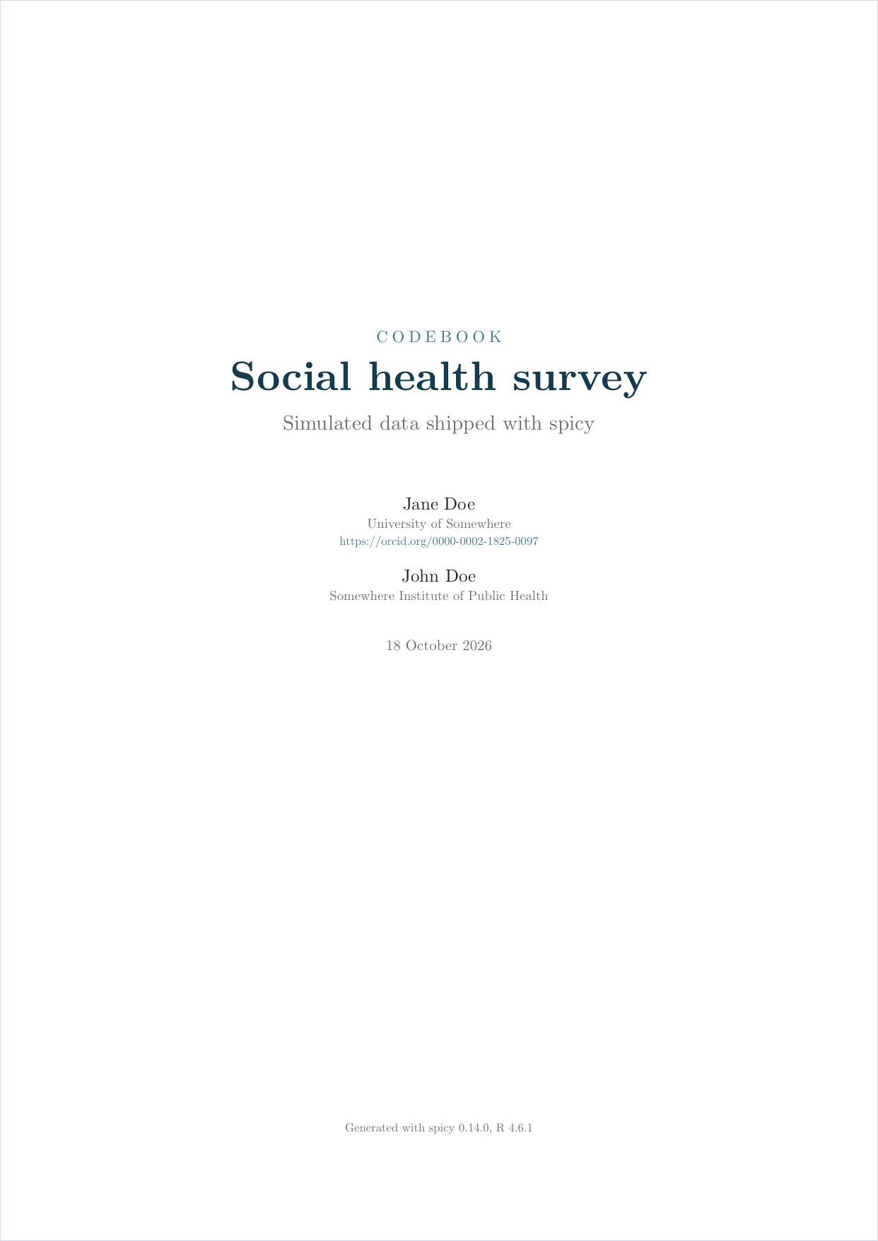
code_book(
  sochealth,
  title = "Social health survey",
  subtitle = "Simulated data shipped with spicy",
  authors = list(
    list(
      name = "Jane Doe",
      affiliation = "University of Somewhere",
      orcid = "0000-0002-1825-0097"
    ),
    list(name = "John Doe", affiliation = "Somewhere Institute of Public Health")
  ),
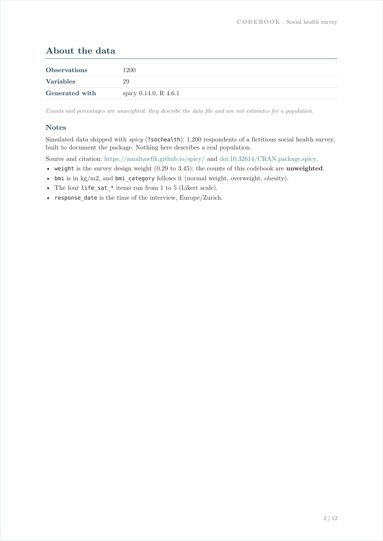
  notes = c(
    "Simulated data shipped with *spicy* (`?sochealth`): 1,200 respondents of a fictitious social health survey, built to document the package. Nothing here describes a real population.",
    "Source and citation: https://amaltawfik.github.io/spicy/ and doi:10.32614/CRAN.package.spicy.",
    "- `weight` is the survey design weight (0.29 to 3.45): the counts of this codebook are **unweighted**.",
    "- `bmi` is in kg/m2, and `bmi_category` follows it (normal weight, overweight, obesity).",
    "- The four `life_sat_*` items run from 1 to 5 (Likert scale).",
    "- `response_date` is the time of the interview, Europe/Zurich."
  ),
  output = "sochealth_codebook.pdf"
)
Three of its twelve pages. The cover:
The page about the data, with the caution on unweighted counts and the notes, their markup rendered and their addresses turned into links:
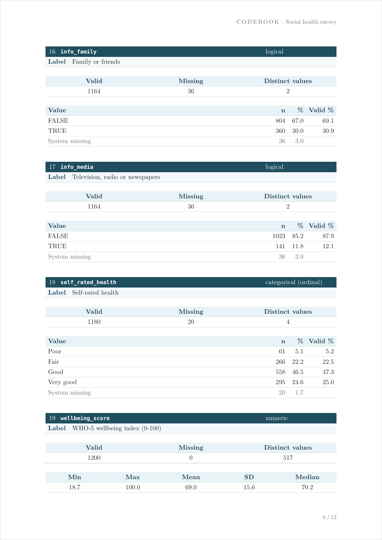
The sheet of self_rated_health, one of the
twenty-nine:
When to use varlist() and code_book()
Use varlist() when you want a quick summary in a script
or a tibble you can inspect directly.
Use vl() when you want the same summary with a shorter
call in interactive work.
Use code_book() when you want a codebook to keep or
share: every variable with the counts of its categories, in an object,
an Excel file, or a PDF.
The two tools differ in one default: varlist() shows
only the observed factor levels in its
Values column (the convention of Stata tab and
of the SPSS FREQUENCIES default, which both list only
values present in the data), whereas code_book() lists
all declared levels in values, unused ones
with a count of 0 – the full coding scheme, as a data dictionary or SPSS
CTABLES would report it. Pass factor_levels =
explicitly to either function to override the default.
Their values arguments differ as well: in
varlist(), values = TRUE prints every value in
the Values column; in code_book(),
values is the maximum number of categories listed per
variable (100 by default).