spicy: APA-style regression and summary tables for R • spicy

spicy is an R package for frequency tables, cross-tabulations, association measures, categorical and continuous summary tables, publication-ready regression tables for 30+ model classes, and labelled survey data workflows.

Features

Every spicy table prints as readable text in the console and exports to gt, tinytable, flextable, Excel, Word, or the clipboard, following APA conventions. Around the tables, spicy provides the survey-data tools that feed them: variable inspection, codebooks, label extraction, and row-wise summaries.

Frequency tables with freq().
Cross-tabulations with cross_tab(): percentages, weights, chi-squared tests, and effect sizes.
Association measures: cramer_v(), phi(), gamma_gk(), kendall_tau_b(), somers_d() and 6 other coefficients; assoc_measures() computes the full set at once.
Categorical and continuous summary tables with table_categorical() and table_continuous(), overall or by group.
Model-based continuous summary tables with table_continuous_lm() for linear-model reporting: classical / HC* / cluster-robust / bootstrap / jackknife variance, four effect-size families (f², Cohen’s d, Hedges’ g, Hays’ omega²) with noncentral CIs, additive covariate adjustment with G-computation (Stata margins style) or equal-weight (emmeans style) marginal means, and weighted comparisons.
Regression tables with table_regression() for one or more fitted models side by side, across 30+ model classes (see Supported models below): classical / heteroskedasticity-robust / cluster-robust / bootstrap / jackknife variance with each class’s field-standard backend, standardised coefficients, family-aware exponentiate (OR / IRR / HR / RR / MR, link-gated), Wald or profile-likelihood CIs, average marginal effects (per-category for ordinal and multinomial models), partial f² / η² / ω² / χ² effect sizes, class-aware fit statistics (pseudo-R², Nakagawa marginal / conditional R², ICC), hierarchical model comparisons with the correct nested test per class, and multiple-comparison adjustment. Mixed models report their random effects as table rows with an optional boundary-correct per-term test; ordinal models report their thresholds; zero-inflated and hurdle models report every model component. Survival models go beyond hazard ratios: adjusted restricted-mean-survival-time and risk differences by g-computation (tau / at_time), for Cox fits (stratified included) and parametric AFT fits, in single tables and in the univariable screen.
Univariable screening with table_regression_uv(): one-predictor-at-a-time models merged with the multivariable fit, per-predictor N and events, for glm, lm, and Cox outcomes.
Variable inspection with varlist() and vl(): names, labels, values, classes, distinct values (N_distinct), valid observations (N_valid), and missing data.
Codebooks with code_book(): interactive and exportable, for labelled and survey-style datasets.
Label extraction with label_from_names(), including LimeSurvey-style headers.
Row-wise summaries with mean_n(), sum_n(), and count_n(), with explicit control over missing values.

Works with labelled, factor, ordered, Date, POSIXct, and other common variable types – and honors declared missing values (haven’s na_values/na_range, tagged NAs) across the descriptive functions, with disclosure notes and a user_na escape hatch. For a full introduction, see Getting started with spicy.

Supported models

table_regression() accepts a single fit or a list of fits from any of these classes, and renders them with the conventions of each model family:

Family	Engines
Linear and generalized linear	`stats::lm()`, `stats::glm()`, `MASS::glm.nb()`, `MASS::rlm()`, `stats::nls()`
Robust, IV, quantile, panel	`estimatr::lm_robust()`, `estimatr::iv_robust()`, `AER::ivreg()`, `AER::tobit()`, `quantreg::rq()`, `fixest::feols()`, `fixest::feglm()`, `fixest::fepois()`, `fixest::fenegbin()`
Mixed effects	`lme4::lmer()`, `lme4::glmer()`, `glmmTMB::glmmTMB()`, `nlme::lme()`, `nlme::gls()`
Ordinal and categorical	`MASS::polr()`, `ordinal::clm()` (incl. partial proportional odds), `nnet::multinom()`, `mlogit::mlogit()`
Counts, two-part models	`pscl::hurdle()`, `pscl::zeroinfl()`, `glmmTMB::glmmTMB()` (zero-inflation and dispersion components)
Survival	`survival::coxph()`, `survival::survreg()`, `rms::cph()`, `flexsurv::flexsurvreg()`
Survey-weighted	`survey::svyglm()` (design-based SEs)
Population-averaged (GEE)	`geepack::geeglm()` (native sandwich SEs, working correlation disclosed)
Additive, proportions, selection	`mgcv::gam()`, `mgcv::bam()`, `betareg::betareg()`, `sampleSelection::selection()`
rms	`rms::ols()`, `rms::lrm()`, `rms::Glm()`
Bayesian	`rstanarm::stan_glm()`, `rstanarm::stan_glmer()`, `brms::brm()` (posterior median, credible intervals, no p-values)

Class-specific structure renders as labelled blocks in the same table: random effects (with SE and CI on each variance component, and an optional boundary-correct per-term likelihood-ratio test), ordinal thresholds, non-proportional effects, zero-inflation and dispersion components. Robust variance requests use each class’s field-standard backend and are refused with a clear message when no valid backend exists.

The full capability map – each family’s marginal-effects estimand, exponentiate semantics, robust-variance backends and standardized-coefficient support – is the Supported models article; table_regression_models() returns the same registry as a data frame.

Installation

Install the current CRAN release, recommended for most users:

install.packages("spicy")

Install the latest r-universe build:

install.packages(
  "spicy",
  repos = c(
    "https://amaltawfik.r-universe.dev",
    "https://cloud.r-project.org"
  )
)

This installs spicy from r-universe when available; CRAN is included only as a fallback for dependencies. The r-universe build may be newer than the current CRAN release.

Install the development version from GitHub with pak:

# install.packages("pak")
pak::pak("amaltawfik/spicy")

Or with remotes:

# install.packages("remotes")
remotes::install_github("amaltawfik/spicy")

Quick tour

The examples below use the bundled sochealth dataset.

Inspect variables

varlist demo with labelled data

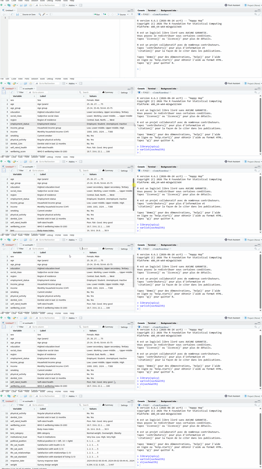
varlist(sochealth, tbl = TRUE)
#> # A tibble: 24 × 7
#>    Variable          Label                 Values Class N_distinct N_valid   NAs
#>    <chr>             <chr>                 <chr>  <chr>      <int>   <int> <int>
#>  1 sex               Sex                   Femal… fact…          2    1200     0
#>  2 age               Age (years)           25, 2… nume…         51    1200     0
#>  3 age_group         Age group             25-34… orde…          4    1200     0
#>  4 education         Highest education le… Lower… orde…          3    1200     0
#>  5 social_class      Subjective social cl… Lower… orde…          5    1200     0
#>  6 region            Region of residence   Centr… fact…          6    1200     0
#>  7 employment_status Employment status     Emplo… fact…          4    1200     0
#>  8 income_group      Household income gro… Low, … orde…          4    1182    18
#>  9 income            Monthly household in… 1000,… nume…       1052    1200     0
#> 10 smoking           Current smoker        No, Y… fact…          2    1175    25
#> # ℹ 14 more rows

code_book(
  sochealth,
  starts_with("bmi"),
  values = TRUE,
  include_na = TRUE
)

See Explore variables and build codebooks for more on varlist(), vl(), and code_book().

Frequency tables and cross-tabulations

freq(sochealth, income_group)
#> Frequency table: income_group
#> 
#>  Category   │ Values            Freq.    Percent    Valid Percent 
#> ────────────┼─────────────────────────────────────────────────────
#>  Valid      │ Low                 247       20.6             20.9 
#>             │ Lower middle        388       32.3             32.8 
#>             │ Upper middle        328       27.3             27.7 
#>             │ High                219       18.2             18.5 
#>  Missing    │ NA                   18        1.5                  
#> ────────────┼─────────────────────────────────────────────────────
#>  Total      │                    1200      100.0            100.0 
#> 
#> Label: Household income group
#> Class: ordered, factor
#> Data: sochealth

cross_tab(sochealth, smoking, education, percent = "col")
#> Crosstable: smoking x education (Column %)
#> 
#>  Values   │   Lower secondary    Upper secondary    Tertiary │   Total 
#> ──────────┼──────────────────────────────────────────────────┼─────────
#>  No       │              69.6               78.7        84.9 │    78.8 
#>  Yes      │              30.4               21.3        15.1 │    21.2 
#> ──────────┼──────────────────────────────────────────────────┼─────────
#>  Total    │             100.0              100.0       100.0 │   100.0 
#>  N        │               257                527         391 │    1175 
#> 
#> Chi-2(2) = 21.6, p <.001
#> Cramer's V = 0.14
#> Missing values removed: smoking (25).

See Frequency tables and cross-tabulations for freq(), cross_tab(), percentages, weights, and tests.

Association measures

tbl <- xtabs(~ self_rated_health + education, data = sochealth)

# Quick scalar estimate
cramer_v(tbl)
#> [1] 0.1761697

# Detailed result with CI and p-value
cramer_v(tbl, detail = TRUE)
#> Estimate  SE  CI lower  CI upper      p
#>    0.176  --     0.120     0.231  <.001

See Cramer’s V, Phi, and association measures for a guide on choosing the right measure.

Summary tables

table_categorical(
  sochealth,
  select = c(smoking, physical_activity),
  labels = c(
    smoking           = "Current smoker",
    physical_activity = "Physical activity"
  )
)
#> Categorical table
#> 
#>  Variable            │   n      %    
#> ─────────────────────┼───────────────
#>  Current smoker      │               
#>    No                │  926    77.2  
#>    Yes               │  249    20.8  
#>    (Missing)         │   25     2.1  
#> ╌╌╌╌╌╌╌╌╌╌╌╌╌╌╌╌╌╌╌╌╌┼╌╌╌╌╌╌╌╌╌╌╌╌╌╌╌
#>  Physical activity   │               
#>    No                │  650    54.2  
#>    Yes               │  550    45.8

table_categorical(
  sochealth,
  select = c(smoking, physical_activity),
  by = education,
  labels = c(
    smoking           = "Current smoker",
    physical_activity = "Physical activity"
  )
)
#> Categorical table by education
#> 
#>  Variable          │ Lower secondary n  Lower secondary %  Upper secondary n 
#> ───────────────────┼─────────────────────────────────────────────────────────
#>  Current smoker    │                                                         
#>    No              │        179               68.6                415        
#>    Yes             │         78               29.9                112        
#>    (Missing)       │          4                1.5                 12        
#> ╌╌╌╌╌╌╌╌╌╌╌╌╌╌╌╌╌╌╌┼╌╌╌╌╌╌╌╌╌╌╌╌╌╌╌╌╌╌╌╌╌╌╌╌╌╌╌╌╌╌╌╌╌╌╌╌╌╌╌╌╌╌╌╌╌╌╌╌╌╌╌╌╌╌╌╌╌
#>  Physical activity │                                                         
#>    No              │        177               67.8                310        
#>    Yes             │         84               32.2                229        
#> 
#>  Variable          │ Upper secondary %  Tertiary n  Tertiary %  Total n 
#> ───────────────────┼────────────────────────────────────────────────────
#>  Current smoker    │                                                    
#>    No              │       77.0            332         83.0       926   
#>    Yes             │       20.8             59         14.8       249   
#>    (Missing)       │        2.2              9          2.2        25   
#> ╌╌╌╌╌╌╌╌╌╌╌╌╌╌╌╌╌╌╌┼╌╌╌╌╌╌╌╌╌╌╌╌╌╌╌╌╌╌╌╌╌╌╌╌╌╌╌╌╌╌╌╌╌╌╌╌╌╌╌╌╌╌╌╌╌╌╌╌╌╌╌╌
#>  Physical activity │                                                    
#>    No              │       57.5            163         40.8       650   
#>    Yes             │       42.5            237         59.2       550   
#> 
#>  Variable          │ Total %    p    Cramer's V 
#> ───────────────────┼────────────────────────────
#>  Current smoker    │          <.001     .14     
#>    No              │  77.2                      
#>    Yes             │  20.8                      
#>    (Missing)       │   2.1                      
#> ╌╌╌╌╌╌╌╌╌╌╌╌╌╌╌╌╌╌╌┼╌╌╌╌╌╌╌╌╌╌╌╌╌╌╌╌╌╌╌╌╌╌╌╌╌╌╌╌
#>  Physical activity │          <.001     .21     
#>    No              │  54.2                      
#>    Yes             │  45.8

table_continuous(
  sochealth,
  select = c(bmi, life_sat_health)
)
#> Descriptive statistics
#> 
#>  Variable                       │   M     SD    Min    Max   95% CI LL 
#> ────────────────────────────────┼──────────────────────────────────────
#>  Body mass index                │ 25.93  3.72  16.00  38.90    25.72   
#>  Satisfaction with health (1-5) │  3.55  1.25   1.00   5.00     3.48   
#> 
#>  Variable                       │ 95% CI UL   n   
#> ────────────────────────────────┼─────────────────
#>  Body mass index                │   26.14    1188 
#>  Satisfaction with health (1-5) │    3.62    1192 
#> 
#> Missing values removed: bmi (12), life_sat_health (8).

table_continuous(
  sochealth,
  select = c(bmi, life_sat_health),
  by = education
)
#> Descriptive statistics
#> 
#>  Variable                       │ Group              M     SD    Min    Max  
#> ────────────────────────────────┼────────────────────────────────────────────
#>  Body mass index                │ Lower secondary  28.09  3.47  18.20  38.90 
#>                                 │ Upper secondary  26.02  3.43  16.00  37.10 
#>                                 │ Tertiary         24.39  3.52  16.00  33.00 
#> ╌╌╌╌╌╌╌╌╌╌╌╌╌╌╌╌╌╌╌╌╌╌╌╌╌╌╌╌╌╌╌╌┼╌╌╌╌╌╌╌╌╌╌╌╌╌╌╌╌╌╌╌╌╌╌╌╌╌╌╌╌╌╌╌╌╌╌╌╌╌╌╌╌╌╌╌╌
#>  Satisfaction with health (1-5) │ Lower secondary   2.71  1.20   1.00   5.00 
#>                                 │ Upper secondary   3.53  1.19   1.00   5.00 
#>                                 │ Tertiary          4.11  1.04   1.00   5.00 
#> 
#>  Variable                       │ Group            95% CI LL  95% CI UL   n  
#> ────────────────────────────────┼────────────────────────────────────────────
#>  Body mass index                │ Lower secondary    27.66      28.51    260 
#>                                 │ Upper secondary    25.73      26.31    534 
#>                                 │ Tertiary           24.04      24.74    394 
#> ╌╌╌╌╌╌╌╌╌╌╌╌╌╌╌╌╌╌╌╌╌╌╌╌╌╌╌╌╌╌╌╌┼╌╌╌╌╌╌╌╌╌╌╌╌╌╌╌╌╌╌╌╌╌╌╌╌╌╌╌╌╌╌╌╌╌╌╌╌╌╌╌╌╌╌╌╌
#>  Satisfaction with health (1-5) │ Lower secondary     2.57       2.86    259 
#>                                 │ Upper secondary     3.43       3.63    534 
#>                                 │ Tertiary            4.01       4.21    399 
#> 
#>  Variable                       │ Group              p   
#> ────────────────────────────────┼────────────────────────
#>  Body mass index                │ Lower secondary  <.001 
#>                                 │ Upper secondary        
#>                                 │ Tertiary               
#> ╌╌╌╌╌╌╌╌╌╌╌╌╌╌╌╌╌╌╌╌╌╌╌╌╌╌╌╌╌╌╌╌┼╌╌╌╌╌╌╌╌╌╌╌╌╌╌╌╌╌╌╌╌╌╌╌╌
#>  Satisfaction with health (1-5) │ Lower secondary  <.001 
#>                                 │ Upper secondary        
#>                                 │ Tertiary               
#> 
#> Missing values removed: bmi (12), life_sat_health (8).

table_continuous_lm(
  sochealth,
  select = c(wellbeing_score, bmi),
  by = sex,
  vcov = "HC3",
  output = "data.frame"
)
#>                                      Variable M (Female) M (Male)
#> wellbeing_score WHO-5 wellbeing index (0-100)   67.16194 71.04879
#> bmi                           Body mass index   25.68506 26.19685
#>                 Δ (Male - Female)  95% CI LL 95% CI UL            p          R²
#> wellbeing_score         3.8868576 2.12265210 5.6510631 1.670572e-05 0.015475137
#> bmi                     0.5117882 0.08904596 0.9345305 1.769614e-02 0.004728908
#>                    n
#> wellbeing_score 1200
#> bmi             1188

fit <- lm(wellbeing_score ~ age + sex + smoking, data = sochealth)
table_regression(fit)
#> Linear regression: wellbeing_score
#> 
#>  Variable        │    B      SE       95% CI        p   
#> ─────────────────┼──────────────────────────────────────
#>  (Intercept)     │   65.20  1.66  [61.95, 68.45]  <.001 
#>  age             │    0.05  0.03  [-0.01,  0.11]   .130 
#>  sex:            │                                      
#>    Female (ref.) │     –     –          –          –    
#>    Male          │    3.86  0.91  [ 2.08,  5.63]  <.001 
#>  smoking:        │                                      
#>    No (ref.)     │     –     –          –          –    
#>    Yes           │   -1.72  1.11  [-3.89,  0.45]   .121 
#> ╌╌╌╌╌╌╌╌╌╌╌╌╌╌╌╌╌┼╌╌╌╌╌╌╌╌╌╌╌╌╌╌╌╌╌╌╌╌╌╌╌╌╌╌╌╌╌╌╌╌╌╌╌╌╌╌
#>  n               │ 1175                                 
#>  R²              │    0.02                              
#>  Adj.R²          │    0.02                              
#> 
#> Note. Linear regression.
#> Std. errors: classical (OLS).

Regression tables cover 30+ model classes with the conventions of each family. A mixed-effects fit, for example, reports its random effects as rows (SD, correlation, residual – each with SE and CI), the ICC and group sizes as fit statistics, and the likelihood-ratio test of the random part with the boundary-correct chi-bar-squared p-value:

library(lme4)
fit_mixed <- lmer(Reaction ~ Days + (Days | Subject), data = sleepstudy)
table_regression(fit_mixed)
#> Linear mixed-effects regression: Reaction
#> 
#>  Variable                        │    B      SE        95% CI         p   
#> ─────────────────────────────────┼────────────────────────────────────────
#>  (Intercept)                     │  251.41  6.82  [238.03, 264.78]  <.001 
#>  Days                            │   10.47  1.55  [  7.44,  13.50]  <.001 
#> ╌╌╌╌╌╌╌╌╌╌╌╌╌╌╌╌╌╌╌╌╌╌╌╌╌╌╌╌╌╌╌╌╌┼╌╌╌╌╌╌╌╌╌╌╌╌╌╌╌╌╌╌╌╌╌╌╌╌╌╌╌╌╌╌╌╌╌╌╌╌╌╌╌╌
#>  Random effects:                 │                                        
#>    σ Subject (Intercept)         │   24.74  5.84  [  6.79,  34.32]   –    
#>    σ Subject Days                │    5.92  1.25  [  2.47,   8.00]   –    
#>    ρ Subject ((Intercept), Days) │    0.07  0.33  [ -0.57,   0.70]   –    
#>    σ (Residual)                  │   25.59  1.51  [ 22.44,  28.39]   –    
#> ╌╌╌╌╌╌╌╌╌╌╌╌╌╌╌╌╌╌╌╌╌╌╌╌╌╌╌╌╌╌╌╌╌┼╌╌╌╌╌╌╌╌╌╌╌╌╌╌╌╌╌╌╌╌╌╌╌╌╌╌╌╌╌╌╌╌╌╌╌╌╌╌╌╌
#>  n                               │  180                                   
#>  N (Subject)                     │   18                                   
#>  R² (marginal)                   │    0.28                                
#>  R² (conditional)                │    0.80                                
#>  AIC                             │ 1755.6                                 
#>  BIC                             │ 1774.8                                 
#> 
#> Note. Linear mixed-effects regression.
#> Std. errors: Wald (model-based).
#> p-values: Wald-z, large-sample approximation. Load `lmerTest` for Satterthwaite t-tests.
#> Random effects (REML): LR test vs linear regression, χ̄²(3) = 150.04, p < .001.

See Categorical summary tables for categorical summaries, Continuous summary tables for continuous summaries and group comparisons, Model-based continuous summary tables for weighted or robust linear-model reporting, Regression coefficient tables for regression tables across model families, and Summary tables for APA-style reporting for an overview of summary tables.

Row-wise summaries

df <- data.frame(
  x1 = c(10, NA, 30, 40, 50),
  x2 = c(5, NA, 15, NA, 25),
  x3 = c(NA, 30, 20, 50, 10)
)

mean_n(df)
#> [1]       NA       NA 21.66667       NA 28.33333
sum_n(df, min_valid = 2)
#> [1] 15 NA 65 90 85
count_n(df, special = "NA")
#> [1] 1 2 0 1 0

See Getting started with spicy for a longer workflow using mean_n(), sum_n(), and count_n().

Label extraction

# LimeSurvey-style headers: "code. label"
df <- tibble::tibble(
  "age. Age of respondent" = c(25, 30),
  "score. Total score" = c(12, 14)
)
out <- label_from_names(df)
labelled::var_label(out)
#> $age
#> [1] "Age of respondent"
#> 
#> $score
#> [1] "Total score"

See Explore variables and build codebooks for more on label_from_names(), varlist(), and code_book().

Documentation

Each workflow has a dedicated vignette:

Key reference pages: freq(), cross_tab(), cramer_v(), table_categorical(), table_continuous(), table_continuous_lm(), table_regression(), varlist(), code_book(), label_from_names(), mean_n(), sum_n(), and count_n() – see the full function index for everything else.

Citation

To cite spicy in a publication or teaching material (this entry is generated by citation("spicy") at build time and always refers to the current CRAN release):

Tawfik A (2026). spicy: Descriptive Statistics, Summary Tables, and Data Management Tools. doi:10.32614/CRAN.package.spicy https://doi.org/10.32614/CRAN.package.spicy. R package version 0.12.0, https://CRAN.R-project.org/package=spicy.

@Manual{,
  title = {spicy: Descriptive Statistics, Summary Tables, and Data Management Tools},
  author = {Amal Tawfik},
  year = {2026},
  note = {R package version 0.12.0},
  url = {https://CRAN.R-project.org/package=spicy},
  doi = {10.32614/CRAN.package.spicy},
}

Package DOI: https://doi.org/10.32614/CRAN.package.spicy.
Source citation file: https://github.com/amaltawfik/spicy/blob/main/inst/CITATION

License

MIT. See LICENSE for details.

spicy: frequency tables, cross-tabulations, summary and regression tables in R